The Low Precision Ephemeris (LPE)

Table of Contents

• Overview
• Idea of the compression
• Organisation of the data
• Precision
• Usage in C
• Usage in Java
• Further development
• Download

Overview

The LPE can be useful in the following areas:

• GUI components where a fast search for planetary positions is needed. Imagine a chart component which allows to move the planet symbols by Drag and Drop. While a symbol is dragged, the LPE can quickly scan forward to find the time when the planet reaches the current position, and the other planets can be redrawn accordingly. When the symbol is dropped, the positions can finally be computed more accurately using a precise library like Swiss Ephemeris.
• When scanning time periods for planetary phenomena like conjunctions, parallels, or ingresses, it may be helpful to precompute the time spans in which the phenomena can only occur. This can be efficiently performed using the LPE. In a second step then, these potential time spans can be analyzed more precise with another ephemeris.

The library is assembled as a DLL which can be included in high-level programming languages like C and Java. For Java, no special wrapper code is necessary, the mapping to Java data is already included in the DLL. See below for details on how to access the LPE from other programs. The DLL file itself is smaller than 10 KBytes. Additionally, ephemeris files with a size of 5 KB per century will be loaded into memory.

Idea of compression

How can this work for an arbitrary century? The planetary perturbations can give errors of several degrees - how can they be taken into respect with such an approach? Ahnert's idea obviously was to put a secular perturbation information into the century's values of his table of mean anomalies, yielding sufficiently good results for many practical purposes. Compared to some brute force approaches using Cebysheff polynomials or the like for a piecewise approximation of the orbit, Ahnert's concept seemed more natural to me, since it builds on the elliptical orbit of the planet and only modifies it slightly by "correcting" the mean anomaly in such a way that the computed position will fit better.

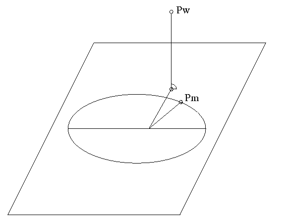
The following figure shows the method I therefore pursued: I projected the true position of a planet (Pw in the figure) on the plane of its mean orbit of date. The projection point has a certain anomaly which can be converted to a corresponding mean anomaly by stepping through the Keplerian procedure to determine the true anomaly in backward direction. This mean anomaly will differ from the mean anomaly that can be computed using the mean orbital elements. These difference terms which I call ΔM values can be computed and saved once in binary data files and then used as corrections in the LPE algorithm.

Similarly, there is a correction term ΔR to obtain the true distance from the Sun from the approximating point on the mean orbit. For each outer planet (Jupiter to Pluto), the values of ΔM and ΔR will be tabulated in 100 day steps. Different to ΔM, the ΔR value will be applied as a factor to the distance after the solution of the Kepler problem.

Organisation of the data

The following assembler definitions document the organization of the first part of the data files (for developers, code will serve better as a documentation than any other text).

; Coefficients for quadratic interpolation
qCoeff struc
  c0     real8 0.  ; intercept
  c1     real8 0.  ; slope
  c2     real8 0.  ; quadratic coefficient
qCoeff ends

; Coefficients for linear interpolation
lCoeff struc
  c0     real8 0.  ; intercept
  c1     real8 0.  ; slope
lCoeff ends

; Orbital elements for linear interpolation
; Each element contains two coefficients - intercept and slope
lOrbEl struc
  a    lCoeff<>  ; semi-axis
  e    lCoeff<>  ; eccentricity
  i    lCoeff<>  ; inclination
  node lCoeff<>  ; ascending node
  peri lCoeff<>  ; perihelion
  M    lCoeff<>  ; mean anomaly
  n    lCoeff<>  ; daily motion
lOrbEl ends

; Orbital elements for quadratic interpolation
; Each elements contains the three coefficents of the parabola
; used for quadratic interpolation
qOrbEl struc
  a    qCoeff<>  ; semi-axis        
  e    qCoeff<>  ; eccentricity     
  i    qCoeff<>  ; inclination      
  node qCoeff<>  ; ascending node   
  peri qCoeff<>  ; perihelion       
  M    qCoeff<>  ; mean anomaly     
  n    qCoeff<>  ; daily motion     
qOrbEl ends

; Pair of 2 Byte Integers: Minimum and Maximum
wordMiniMax struc
  min dw ?
  max dw ?
wordMiniMax ends

; Minima and Maxima of r and m
rmMiniMax struc
  m wordMiniMax<>
  r wordMiniMax<>
rmMiniMax ends

; Minima und Maxima of the r and m values contained in the file
MiniMax struc
  jup    rmMiniMax<>
  sat    rmMiniMax<>
  ura    rmMiniMax<>
  nep    rmMiniMax<>
  plu    rmMiniMax<>
MiniMax ends

; Structure of the file
fileStruc struc
  jd0      db 3 dup(0)   ; 3-byte int: Julian start date
  jd1      db 3 dup(0)   ; 3-byte int: Julian end date
  incr     db 2 dup(0)   ; 2-byte int: increment in days
  mer      lOrbEl<>
  ven      lOrbEl<>
  mar      lOrbEl<>
  jup      qOrbEl<>
  sat      qOrbEl<>
  ura      qOrbEl<>
  nep      qOrbEl<>
  plu      qOrbEl<>
  minimax  MiniMax<>
  data     db 0 ; From here on, the bit field for delta M / delta R values start
fileStruc ends

Precision

These figures being in scope for the current century, the differences deteriorate quickly when leaving this time range, as the following table shows. It gives the maximum deviations for each planet per century file. The deviations increase when going to the past - up to values of about 1 degree in 50 C.E. There seems to be a systematic secular error which should be analyzed in a future release. One source of the error clearly is the fixed orbit for the earth, copied from Montenbruck's Grundlagen der Ephemeridenrechnung, but this contributes with only 6' in 50 C.E. Also, the analytical moon theory used seems to be optimized for the current times.

Maximum deviations (in ' of arc) of computed positions

Start year	Sun	Moon	Mercury	Venus	Mars	Jupiter	Saturn	Uranus	Neptune	Pluto
2050	1.051	1.844	1.418	2.703	5.783	0.743	0.687	0.675	0.687	1.130
1950	1.107	1.725	1.469	2.614	4.328	0.741	0.718	0.696	0.667	1.418
1850	1.112	1.660	1.392	2.800	3.840	0.733	0.715	0.677	0.665	1.288
1750	1.163	1.928	1.393	2.674	3.170	0.729	0.684	0.722	0.703	0.936
1650	1.003	1.885	1.400	2.413	3.229	0.727	0.686	0.686	0.661	0.915
1550	0.951	3.049	1.188	1.867	2.819	0.688	0.688	0.696	0.663	0.836
1450	0.832	3.862	1.500	1.658	3.622	0.677	0.639	0.675	0.665	1.783
1350	0.932	5.829	1.826	2.474	5.057	0.655	0.643	0.664	0.646	1.714
1250	1.133	7.892	1.934	3.276	4.997	0.585	0.615	0.639	0.644	0.944
1150	1.413	9.924	2.569	4.259	6.135	0.533	0.592	0.622	0.637	1.004
1050	1.655	13.009	2.761	5.257	6.362	0.525	0.588	0.630	0.643	0.785
950	1.994	15.708	3.442	6.430	7.266	0.472	0.539	0.611	0.610	1.952
850	2.250	19.008	4.019	7.294	8.722	0.424	0.512	0.590	0.631	1.932
750	2.619	23.143	4.820	8.466	8.429	0.561	0.492	0.587	0.614	0.932
650	3.022	26.500	5.341	10.193	8.594	0.696	0.456	0.534	0.591	0.950
550	3.452	30.882	5.870	11.593	9.775	0.725	0.421	0.545	0.588	0.689
450	3.894	35.709	6.986	13.996	10.859	0.867	0.409	0.527	0.550	1.837
350	4.558	40.333	7.985	15.156	11.829	0.961	0.432	0.491	0.547	0.660
250	5.118	46.161	8.826	17.869	13.899	1.157	0.511	0.476	0.549	1.016
150	5.787	51.393	9.877	19.467	14.861	1.314	0.583	0.418	0.516	0.825
50	6.429	57.314	11.489	22.428	16.109	1.488	0.661	0.435	0.490	0.663

Usage in C (or other languages)

int lpeGetPlanet( unsigned int pPlanet, double pJD, double* pLBR);
int lpeGetPlanets( double pJD, double* pLBR);
int lpeSetDirectory( char* dir );  

• lpeGetPlanet computes planet pPlanet at ephemeris time as Julian date pJD, giving back the three geocentric coordinates longitude, latitude and distance in AU referred to the equator and ecliptic of date. The argument pLBR must be a pointer to an array with at least 3 doubles. The integer return code is zero if the computation was successful - it has a value <>0 if an error occurred (i.e. the ephemeris file could not be found or the Julian date is out of the accepted range).
• lpeGetPlanets is like lpeGetPlanet, but computes Sun, Moon and all the planets as a set. The argument pLBR must be a pointer to an array with at least 30 doubles.
• lpeSetDirectory can be used to set the directory where the data files J1950.dat etc. reside. If the function is not called, the library works with the current directory at execution.

Usage in Java

The following code contains the minimum code to make the LPE accessible for Java calls. The functions can then be called as static methods like LpeLoader.lpeGetPlanets() and so on.

class LpeLoader {
  
// at class load, locate and load the LPE library
  static {
    System.loadLibrary("lpe");
    }
    
    
// Available functions from the library
  public static native int lpeGetPlanet(int ipl, double jd, double[] LPR);
  public static native int lpeGetPlanets(double jd, double[] coor);
  public static native int lpeSetDirectory(String dir);
    
}

Further development

There is a GNU makefile containing the build instructions for lpe.dll and a test program lpe_test.exe which will be assembled and executed automatically with each build of lpe.dll.

The output of lpe_test.exe accords to the very simple Test Anything Protocol (TAP). If everything went fine, it looks like this:

1..23
ok 1
ok 2
[ and so on: ok 3, ok 4, ...]
ok 23

For future releases, the following items will be considered:

• Optimization of the data file structure. For reasons of compatibility with the Java class LowPrecCalculator, the data file structure has not been touched in release 1.1. For future releases, the assembler library can go different ways than the Java class, enabling optimization of the file structure. I collect some optimizations worth to be considered.
• The 8-byte swap for the floating-point numbers can be saved. The Big Endian format was only necessary for making the data readable as a Java double by direct file access.
• Currently, the members of the bit field for ΔM and ΔR are of variable length, the length differing for each file, depending on the maximum and minimum values for ΔM and ΔR. Working with members of fixed overall bit size for each member might improve performance in reading it.
• It should be analyzed which elements for which planet really require a linear or even quadratic regression. If the values for an element oscillate very strongly (as is the case for semi-axis and eccentricity) a constant value for the time span should be sufficient.
• The Mars ephemeris should be improved to a precision better than 1' of arc for the longitude. The only way to achieve this will probably be to work with ΔM and ΔR values, as we used them for Jupiter, Saturn, Uranus, Neptune and Pluto.
• The systematic error in the Earth orbit increasing in the past should be eliminated. The elements for the Earth orbit can be added to the Ephemeris file. This has effect on the positions of the other planets, since finally the functions return geocentric coordinates.
• The Moon ephemeris should be replaced by an analytical theory which is accurate to a minute of arc over the whole time span.
• The ephemeris should be extended to handle an arbitrary set of objects (instead of the actual set Sun, Moon, Mercury, ... Pluto). This is a requirement for the Ephemeris Compiler, the program to obtain the condensed data files J1950.dat etc. But the necessary change in the definition of the data files, providing a flexible definition of the contained objects, will of course also require to change the reading of the data in the LPE itself.

Download

For download and for all information around this project, visit the Project Page.

The development is under the GNU public license.